

9. Scraping and Mapping Geographical Data
- Apr 26, 2020
- 13 min read
Updated: Apr 27, 2020
1. Preface
First of all, just like the last post, take a look at the figure below.
This is a map of 18 species of Arecaceae - palm trees - created using Plotly with Python. While the map by default shows all species in the data, you can choose which species to display by selecting them in the drop down menu at the top left. You can also zoom in and out using the control at the top right, as well as change the theme of the map with the tab on the bottom right. The map looks sleek thanks to the mapbox attribute being used in the code. Maps like this will make your data presentation impressive for sure. And, as you might have guessed, we are going to learn how to make it in the following.
Palm trees, a genus typically found in the tropical region, have drawn attention not only from resort developers and business owners of coconut products but also from environmental scientists, as their northward distribution might indicate an increase of the global temperature. This 2018 study published by Nature examined exactly that indeed. In the analysis, the researchers used a relatively large data set of palm trees, which is an open source available to all of us; the map above visualizes part of it.
If you are someone working on biodiversity, you might be familiar with the database Global Biodiversity Information Facility (GBIF). As of writing this article, there are over 52,000 data sets, and more than 4,300 peer-reviewed papers have utilized the database. The user needs to create an account but the process is very easy.
The Arecaceae (palm tree) data table can be found in this page. Currently, there are nearly 100,000 observations in the table. The page also has a built-in map showing the locations of each observation in the table. If you have wondered how those maps are made but are yet to check it out, now is the time. Let's dive in without further ado.
2. Data Collection
In this project, we are going to use the data found on the link right above. First, we need to get the data table. One way to do so is simply downloading the files from the page (there is a download button). I tried this in the beginning... but it didn't work for me. The data came in a text file where the columns and rows were scattered around where I could hardly see a structure. We need to employ an alternative method.
That's why, along data mapping, we are also learning web scraping in this project. We are incredibly lucky, since there is a tutorial by Dr. Wyatt Sharber, a contributor at Medium, on how to scrape data using GBIF's API with Python. We can just modify the codes he shares a little to get the data of our interest. Let's take a look at the modified code:
# Get the data.
import requests
import pandas as pd

base_url = "https://api.gbif.org/v1/occurrence/search?"

def get_GBIF_response(base_url, offset, params, df):
    """Performs an API call to the base URL with additional parameters listed in 'params'. Concatenates response to a Pandas DataFrame, 'df'."""

    #Construct the query URL
    query = base_url+'&'+f'offset={offset}'
    for each in params:
        query = query+'&'+each

    #Call API
    response = requests.get(query)

    #If call is successful, add data to df
    if response.status_code != 200:
        print(f"API call failed at offset {offset} with a status code of {response.status_code}.")
    else:
        result = response.json()
        df_concat = pd.concat([df, pd.DataFrame.from_dict(result['results'])], axis = 0, ignore_index = True, sort = True)
        endOfRecords = result['endOfRecords']
        return df_concat, endOfRecords, response.status_code
    #set parameters for API call
    params = ['limit=300', 'taxon_key=7681', 'hasCoordinate=true',
    'hasGeospatialIssue=false']
    #Set up a simple while loop to continue downloading until the last page
    df = pd.DataFrame()
    endOfRecords = False
    offset = 0
    status = 200
    while endOfRecords == False and status == 200:
        df, endOfRecords, status = get_GBIF_response(base_url, offset, params, df)
        offset = len(df) + 1
As usual, we start by loading necessary modules. After setting base_url which is identical over the entire iterative process, define the repetitive function called get_GBIF_response. The terms in the parentheses, i.e., base_url, offset, params, df, are the key variables here.
Explaining the code line by line would be verbose and confusing. Even if you are not familiar with Python, you could get a pretty good understanding along the following synopsis. Basically, the code repeats the following tasks.
1. Python starts searching a page with base_url. As set by the function query, the text "offset=" and an offset value defined later follow base_url, except for the first round.
2. Then, Python requests data according to params. The number of occurrences (rows of the table) displayed in a page is set at 300, the maximum number (20 by default: you can see that for yourself here). The text "taxon_key=7681" is added after the offset (right after base_url in the first round) and Python sends a request for data to GBIF's server. If there is no problem in accessing it, Python receives a status code of "200" meaning "OK" in HTTP lingo. If a status code of any other value is sent, that means there is a problem and data cannot be accessed; Python would report an error saying: "API call failed at offset {offset} with a status code of {response.status_code}".
3. If the status code is 200, Python checks if the occurrence (row) has coordinates and is free from geo-spatial issues by two boolean variables hasCoordinate and hasGeospatialIssue. Either hasCoordinate is false or hasGeospatialIssue is true, the occurrence is ignored (because they are not useful for mapping) and Python moves on to the next row. If there are the coordinates and there is no issue, then Python stores the row into df (data frame).
4. If the end of records is not reached within 300 rows on the page, Python moves on to the next page by adding 300 to the offset and goes back to 1. in loop until it reaches the end of records.
Actually, the code runs in milliseconds and the data set of 100,000 will be stored in the memory before you notice. Save the data as a CSV file with the following code:
# Save data as a CSV file for cleanup.
df.to_csv(r'C:\Users\Norrie\Palm Trees\Arecaceae.csv', index = False)
Sweet, we are now done with the data collection. The CSV can be found in this page in my repository.
3. Data Cleaning and More
Data cleaning process for this project is very simple as we deal with only one table.
Open the CSV file with Excel and delete columns that are not useful. You can find the cleaned up version of the table here.
There is a few more things we need to do for preparation, though. The maximum size of a file that can be handled by a free account of Plotly is 5M byte while our table is over 40M byte. That means we cannot map all of our 100,000 palm tree observations together and have to make multiple maps each of which containing certain species.
Considering the size limit for each map, I made a list of species in the table using this function in Excel and divided the table into 9 files for the following groups of species with some operation carried out in this file:
Map Data 1_Acanthophoenix to Astrocaryum (Data in the map at the top of this page):
Acanthophoenix, Acoelorraphe, Acoelorrhaphe, Acrocomia, Actinokentia, Adonidia, Aiphanes, Allagoptera, Ammandra, Ancistrophyllum, Aphandra, Archontophoenix, Areca, Arecaceae, Arecastrum, Arenga, Asterogyne, Astrocaryum.
Map Data 2_Attalea
Attalea Map Data 2_Bactris (It should have been "Map Data 3". I noticed the mistake much later but it has no practical implications so I let it be):
Bactris
Map Data 3_Balaka to Cocos
Balaka, Barcella, Basselinia, Beccariophoenix, Bismarckia, Borassodendron, Borassus, Brahea, Brassiophoenix, Burretiokentia, Butia, Calamus, Calyptrocalyx, Calyptrogyne, Calyptronoma, Carpentaria, Caryota, Ceroxylon, Chamaedorea, Chamaedoreaceae, Chamaedrea, Chamaerops, Chelyocarpus, Chrysalidocarpus, Chuniophoenix, Clinosperma, Coccothrinax, Cocos
Map Data 4_Colpothrinax to Gaussia
Colpothrinax, Copernicia, Corypha, Cryosophila, Cyrtostachys, Daemonorops, Deckenia, Desmoncus, Dictyocaryum, Dictyosperma, Drymophloeus, Dypsis, Elaeis, Eleiodoxa, Eremospatha, Erythea, Eugeissona, Euterpe, Gaussia Map Data 5_Guihaia to Nypa
Guihaia, Gulubia, Hedyscepe, Hemithrinax, Heterospathe, Howea, Hydriastele, Hyophorbe, Hyospathe, Hyphaene, Iguanura, Iriartea, Iriartella, Itaya, Jailoloa, Johannesteijsmannia, Juania, Jubaea, Jubaeopsis, Kentia, Kerriodoxa, Korthalsia, Laccospadix, Laccosperma, Lanonia, Latania, Lemurophoenix, Leopoldinia, Lepidocaryum, Lepidorrhachis, Leucothrinax, Licuala, Linospadix, Livistona, Lodoicea, Lytocaryum, Manicaria, Marojejya, Masoala, Mauritia, Mauritiella, Medemia, Metroxylon, Myrialepis, Nannorrhops, Nenga, Neonicholsonia, Nephrosperma, Normanbya, Nypa
Map Data 6_Oenocarpus to Rhapis
Oenocarpus, Oncocalamus, Oncosperma, Orania, Oraniopsis, Palmae, Parajubaea, Phoenicophorium, Phoenix, Pholidostachys, Physokentia, Phytelephas, Pigafetta, Pinanga, Plectocomia, Plectocomiopsis, Podococcus, Polyandrococos, Prestoea, Pritchardia, Pseudophoenix, Ptychococcus, Ptychosperma, Raphia, Ravenea, Reinhardtia, Rhapidophyllum, Rhapis Map Data 7_Rhopaloblaste to Syagrus
Rhopaloblaste, Rhopalostylis, Roscheria, Roystonea, Sabal, Sabinaria, Salacca, Saribus, Satranala, Scheelea, Schippia, Sclerosperma, Serenoa, Socratea, Solfia, Sommieria, Syagrus Map Data 8_Synechanthus to Wodyetia
Synechanthus, Tahina, Thrinax, Trachycarpus, Trithrinax, Veitchia, Verschaffeltia, Voanioala, Wallichia, Washingtonia, Welfia, Wendlandiella, Wettinia, Wodyetia
The species Geonoma had to be excluded from the list since the species alone has a too large number of observations, most of which are found in Peru, to be mapped. These separate files can be found in my repository as well.
Next, create the following three-line code for each species in the column next to the list of species; we'll use it in the mapping code later:
            dict(label = 'Species_Name',
                 method = 'update',
                 args = [{'visible': [False, False, False, False, False, False, False, False, False, False, False, False, False, False, False, False, False, False]}]),
It can be created repeatedly with different Species_Names using the list made above and some Excel formula including this one for line breaking:
=" dict(label = '"&C2&"',"&CHAR(10)&" method = 'update',"&CHAR(10)&" args = [{'visible': [False, False, False, False, False, False, False, False, False, False, False, False, False, False, False, False, False, False]}]),"I wrote this script in the cell D2, which is right next to the list of species, and as you can see, in the formula I referred to cell C2, which holds the first entry of the species list. Once you wrote the script referring to the first species, i.e., Acanthophoenix, you can duplicate the formula with the corresponding referent all the way down to the 177th species, Wodyetia.
These cells, however, contain the formula and not the code part we want to insert into Python code itself. That's why we copy the cells from D2 to D178 in this demonstration and paste the values in column E (how to paste values of copied cells was discussed in my previous post). The figure below shows how it looks like in Excel:
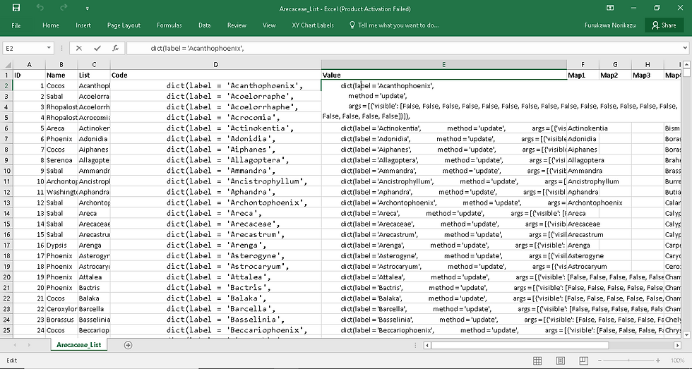
If you copy and paste the cells in column E directly to Python, quite annoyingly, double quotation marks will be added to the beginning and end of each cell content. In order to avoid that, first, paste the cells to a Notepad, then press Ctrl + H and click on Replace All to delete all double quotation marks (this may be a good reason for us to use single quotation marks in codes: otherwise, necessary quotation marks would be deleted as well). You must have just made this text file.
It's been a lot of work already lol
But we just got ready for mapping the data!
4. Data Mapping
Once prepared with the data, we can map them using Plotly with Python. If you have not installed Plotly yet, you can find the instruction for that (it's a bit complicated) in my previous post.
For the mapping, we can modify the code shared in this tutorial by Ms. Emma Grimaldi, another contributor at Medium. The following is the code for mapping the file Map Data 1_Acanthophoenix to Astrocaryum (I didn't color the commands here; that would take too much time):
# Import Plotly to map the data with mapbox tools (create Username, API key, and Access Token at Plotly and mapbox following the aforementioned tutorial by Emma).
import pandas as pd
import chart_studio as py
import plotly.graph_objs as go
from chart_studio.plotly import iplot
import plotly
import pandas as pd

# Setting user, api key and access token
py.tools.set_credentials_file(username='NorrieF', api_key='jVf7ynJyxiVAHGsmfjtS')
mapbox_access_token = 'pk.eyJ1Ijoibm9ycmllZiIsImEiOiJjazlkanB6czIwNGZ3M3BzNjdrMXFlemo1In0.S3Nd5-tLrwK7hLTffw3vTw'

# Load the cleaned up version of Arecaceae.csv
df = pd.read_csv(r"C:\Users\Norrie\Palm Trees\Map Data 1_Acanthophoenix to Astrocaryum.csv", encoding='latin-1')

# Create a list of species from the unique values of the column "Name" in the dataframe
species = df.Name.unique()

# Define the data to show.
data = []
for i in species:
    palm_data = dict(
            lat = df.loc[df['Name'] == i,'Latitude'],
            lon = df.loc[df['Name'] == i,'Longitude'],
            name = i,
            marker = dict(size = 8, opacity = 0.5),
            type = 'scattermapbox'
        )
    data.append(palm_data)

# Lay out the map.
layout = dict(
    height = 800,
    # top, bottom, left and right margins
    margin = dict(t = 0, b = 0, l = 0, r = 0),
    font = dict(color = '#FFFFFF', size = 11),
    paper_bgcolor = '#000000',
    mapbox = dict(
        # here you need the token from Mapbox
        accesstoken = mapbox_access_token,
        bearing = 0,
        # where we want the map to be centered
        center = dict(
            lat = 35,
            lon = -140
        ),
        # we want the map to be "parallel" to our screen, with no angle
        pitch = 0,
        # default level of zoom
        zoom = 1,
        # default map style
        style = 'dark'
    )
)

# Define the contents of the map.
updatemenus=list([
    # drop-down 1: map styles menu
    # buttons containes as many dictionaries as many alternative map styles I want to offer
    dict(
        buttons=list([
            dict(
                args=['mapbox.style', 'dark'],
                label='Dark',
                method='relayout'
            ),
            dict(
                args=['mapbox.style', 'light'],
                label='Light',
                method='relayout'
            ),
            dict(
                args=['mapbox.style', 'outdoors'],
                label='Outdoors',
                method='relayout'
            ),
            dict(
                args=['mapbox.style', 'satellite-streets'],
                label='Satellite with Streets',
                method='relayout'
            )
        ]),
        # direction where I want the menu to expand when I click on it
        direction = 'up',

        # here I specify where I want to place this drop-down on the map
        x = 0.985,
        xanchor = 'left',
        y = 0.1,
        yanchor = 'bottom',

        # specify font size and colors
        bgcolor = '#000000',
        bordercolor = '#FFFFFF',
        font = dict(size=11)
    ),

    # drop-down 2: select species of palm trees to visualize
    dict(
         # for each button I specify which dictionaries of my data list I want to visualize. Remember I have 7 different
         # types of storms but I have 8 options: the first will show all of them, while from the second to the last option, only
         # one type at the time will be shown on the map
         buttons=list([
            dict(label = 'All Species',
                 method = 'update',
                 args = [{'visible': [True, True, True, True, True, True, True, True, True, True, True, True, True, True, True, True, True, True]}]),
            dict(label = 'Acanthophoenix',
                 method = 'update',
                 args = [{'visible': [True, False, False, False, False, False, False, False, False, False, False, False, False, False, False, False, False, False]}]),
            dict(label = 'Acoelorraphe',
                 method = 'update',
                 args = [{'visible': [False, True, False, False, False, False, False, False, False, False, False, False, False, False, False, False, False, False]}]),
            dict(label = 'Acoelorrhaphe',
                 method = 'update',
                 args = [{'visible': [False, False, True, False, False, False, False, False, False, False, False, False, False, False, False, False, False, False]}]),
            dict(label = 'Acrocomia',
                 method = 'update',
                 args = [{'visible': [False, False, False, True, False, False, False, False, False, False, False, False, False, False, False, False, False, False]}]),
            dict(label = 'Actinokentia',
                 method = 'update',
                 args = [{'visible': [False, False, False, False, True, False, False, False, False, False, False, False, False, False, False, False, False, False]}]),
            dict(label = 'Adonidia',
                 method = 'update',
                 args = [{'visible': [False, False, False, False, False, True, False, False, False, False, False, False, False, False, False, False, False, False]}]),
            dict(label = 'Aiphanes',
                 method = 'update',
                 args = [{'visible': [False, False, False, False, False, False, True, False, False, False, False, False, False, False, False, False, False, False]}]),
            dict(label = 'Allagoptera',
                 method = 'update',
                 args = [{'visible': [False, False, False, False, False, False, False, True, False, False, False, False, False, False, False, False, False, False]}]),
            dict(label = 'Ammandra',
                 method = 'update',
                 args = [{'visible': [False, False, False, False, False, False, False, False, True, False, False, False, False, False, False, False, False, False]}]),
            dict(label = 'Ancistrophyllum',
                 method = 'update',
                 args = [{'visible': [False, False, False, False, False, False, False, False, False, True, False, False, False, False, False, False, False, False]}]),
            dict(label = 'Aphandra',
                 method = 'update',
                 args = [{'visible': [False, False, False, False, False, False, False, False, False, False, True, False, False, False, False, False, False, False]}]),
            dict(label = 'Archontophoenix',
                 method = 'update',
                 args = [{'visible': [False, False, False, False, False, False, False, False, False, False, False, True, False, False, False, False, False, False]}]),
            dict(label = 'Areca',
                 method = 'update',
                 args = [{'visible': [False, False, False, False, False, False, False, False, False, False, False, False, True, False, False, False, False, False]}]),
            dict(label = 'Arecaceae',
                 method = 'update',
                 args = [{'visible': [False, False, False, False, False, False, False, False, False, False, False, False, False, True, False, False, False, False]}]),
            dict(label = 'Arecastrum',
                 method = 'update',
                 args = [{'visible': [False, False, False, False, False, False, False, False, False, False, False, False, False, False, True, False, False, False]}]),
            dict(label = 'Arenga',
                 method = 'update',
                 args = [{'visible': [False, False, False, False, False, False, False, False, False, False, False, False, False, False, False, True, False, False]}]),
            dict(label = 'Asterogyne',
                 method = 'update',
                 args = [{'visible': [False, False, False, False, False, False, False, False, False, False, False, False, False, False, False, False, True, False]}]),
            dict(label = 'Astrocaryum',
                 method = 'update',
                 args = [{'visible': [False, False, False, False, False, False, False, False, False, False, False, False, False, False, False, False, False, True]}]),
        ]),
        # direction where the drop-down expands when opened
        direction = 'down',
        # positional arguments
        x = 0.00,
        xanchor = 'left',
        y = 0.99,
        yanchor = 'bottom',
        # fonts and border
        bgcolor = '#000000',
        bordercolor = '#FFFFFF',
        font = dict(size=11)
    )
])

# Assign the list of dictionaries to the layout dictionary.
layout['updatemenus'] = updatemenus

# Decide the title
title = go.layout.Title(text = "Palm Tree World Map (Species: Acanthophoenix to Astrocaryum)", x = 0.5)
# Add the title.
layout['title'] = title

# Generate the map.
figure = dict(data = data, layout = layout)
iplot(figure, filename = 'Palm Tree World Map (Species: Acanthophoenix to Astrocaryum) by Norrie')
If the code is hard to read, you can find the complete code for the 9 maps in a Jupyter Notebook in this page.
The code is pretty long. But the most important feature is the drop-down button. There, you can see that we are using the three-line codes prepared earlier in Notepad. The first choice among the drop-down is "All Species" to display every observation in the table, so the argument that a particular species is "visible" is True for all. The second choice shows only the first species (Acanthophoenix) and nothing else; the argument is False for all but the first entity. Following the same logic, we will reach the last species (Astrocaryum) with the argument True only for itself. When you are done, you will see an identity matrix (True in the diagonal and False elsewhere else) formed underneath the segment for "All Species". The dimension of the identity matrix will differ for tables according to the number of species.
You can study the rest of code by examining it carefully and compare it with the output map. Emma's tutorial will help too. Anyway, you will see the map at the top of this page running this code, and you can save and embed it in any website in the way explained in this post. Congrats! By modifying it slightly, you can display any table of data that come with coordinates. What are you going to map?
5. Postface
I created 9 maps using this code in Jupyter Notebook. They had to be stored in individual repositories and titled "index.html" to be ready for embedding elsewhere. While the first map is shown at the beginning of this page, you can see other maps at the following links.
Why did I choose palm trees for this data mapping exercise? You might have guessed... as I mentioned at the end of the last post, I am starting to work, and yes, it's has to do with palm trees. In a nearby neighborhood, I found a dealer of palm trees, and I will start working with them. Because I want to learn more about the species, the future data science series in this blog will use palm tree data as an example. I'm sorry if you have no interest in the kind of tree (but I believe most people love the tree), but still, the methods I'm sharing here will be very useful for all doing data analysis.
Anyway, please Iook forward to the next post. Until then, keep up with the metrics!


Comments